Waffle chart for time evolution

NoteCredit

This reproduces a visualization created by Muhammad Azhar for the #30DayChartChallenge, as featured on the R Graph Gallery. Data: NOAA (the storms dataset bundled with the tidyverse). All credit for the original design goes to the author.

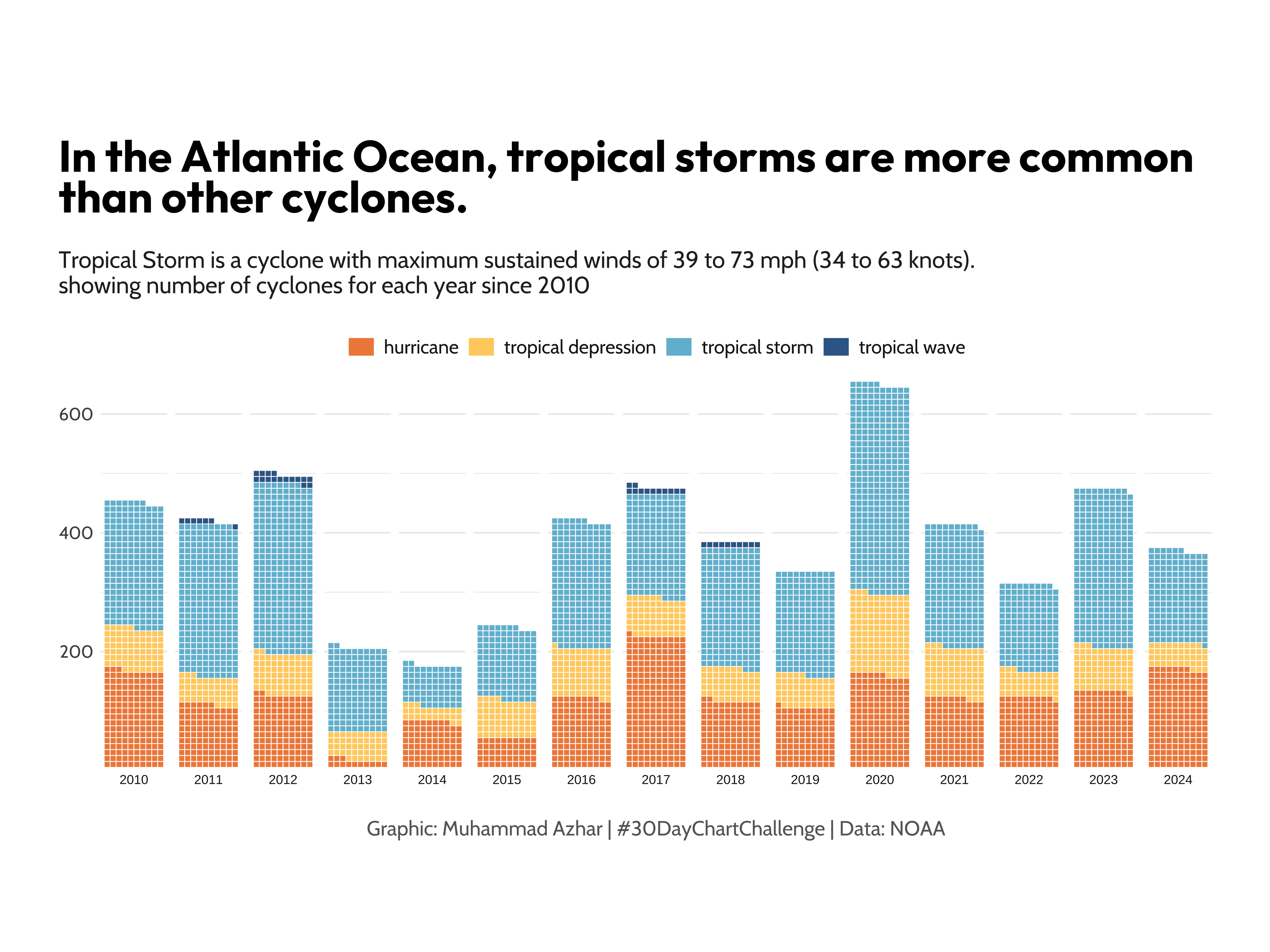
A waffle chart showing how the yearly count of Atlantic tropical cyclones, split by storm category, has evolved since 2010.

library(tidyverse)
library(showtext)
library(ggtext)
library(waffle)
library(MetBrewer)

# Load fonts
font_add_google("Outfit", "title_font")
font_add_google("Cabin", "body_font")
showtext_auto()
title_font <- "title_font"
body_font <- "body_font"

# Prepare data
storms_df <- storms |>
  filter(year >= 2010,
         status %in% c("hurricane", "tropical depression",
                       "tropical storm","tropical wave")) |>
  count(year, status)

# Define text labels
title_text <- "In the Atlantic Ocean, tropical storms are more common than other cyclones."
subtitle_text <- "Tropical Storm is a cyclone with maximum sustained winds of 39 to 73 mph (34 to 63 knots).\nshowing number of cyclones for each year since 2010"
caption_text <- "Graphic: Muhammad Azhar | #30DayChartChallenge | Data: NOAA"

# Create waffle chart
ggplot(storms_df, aes(fill = status, values = n)) +
  geom_waffle(color = "white", size = .25, n_rows = 10, flip = TRUE) +
  facet_wrap(~year, nrow = 1, strip.position = "bottom") +
  scale_x_discrete() +
  scale_y_continuous(labels = function(x) x * 10,
                     expand = c(0,0)) +
  MetBrewer::scale_fill_met_d("Hiroshige", direction=1) +
  coord_equal() +
  labs(title = title_text,
       subtitle = subtitle_text,
       caption = caption_text) +
  theme_minimal() +
  theme(
    axis.title = element_blank(),
    axis.text.x = element_text(family = body_font, size=12),
    axis.text.y = element_text(family = body_font, size=12),
    legend.position = "top",
    legend.title = element_blank(),
    legend.spacing = unit(0.5, 'cm'),
    legend.key.height = unit(0.5, 'cm'),
    legend.key.width = unit(0.7, 'cm'),
    legend.text = element_text(family = body_font, size=13, face = 'plain', color = "grey10"),
    plot.title.position = "plot",
    plot.title = element_textbox(margin = margin(20, 0, 10, 0), size = 30,
                                 family = title_font, face = "bold", width = unit(55, "lines")),
    plot.subtitle = element_text(margin = margin(10, 0, 20, 0), size = 16,
                                 family = body_font, color = "grey15"),
    plot.caption = element_text(family=body_font, face="plain", size=14,
                                color="grey40", hjust=.5, margin=margin(20,0,0,0)),
    plot.background = element_rect(color="white", fill="white"),
    plot.margin = margin(20, 40, 20, 40)
  )

How it is built, step by step

Each tab adds one layer of the recipe on top of the previous one, so you can see what every piece of the final chart contributes. The code for each step is shown below its plot.

1. Counting storms

The data work is a single count(): one row per year and storm status, which is all geom_waffle() needs. Every square in the finished chart stands for one cyclone.

# A tibble: 8 × 3
   year status                  n
  <dbl> <fct>               <int>
1  2010 hurricane             163
2  2010 tropical depression    72
3  2010 tropical storm        212
4  2011 hurricane             106
5  2011 tropical depression    47
6  2011 tropical storm        256
7  2011 tropical wave           7
8  2012 hurricane             122

head(storms_df, 8)

2. Squares

waffle::geom_waffle() turns those counts into squares. Without faceting all years are pooled into one block, stacked ten squares high.

w2 <- ggplot(storms_df, aes(fill = status, values = n)) +
  geom_waffle(color = "white", size = .25, n_rows = 10, flip = TRUE)
w2

3. One block per year

facet_wrap() with nrow = 1 splits the squares into a column per year and moves the year labels to the bottom, which is what makes the chart read as a time series.

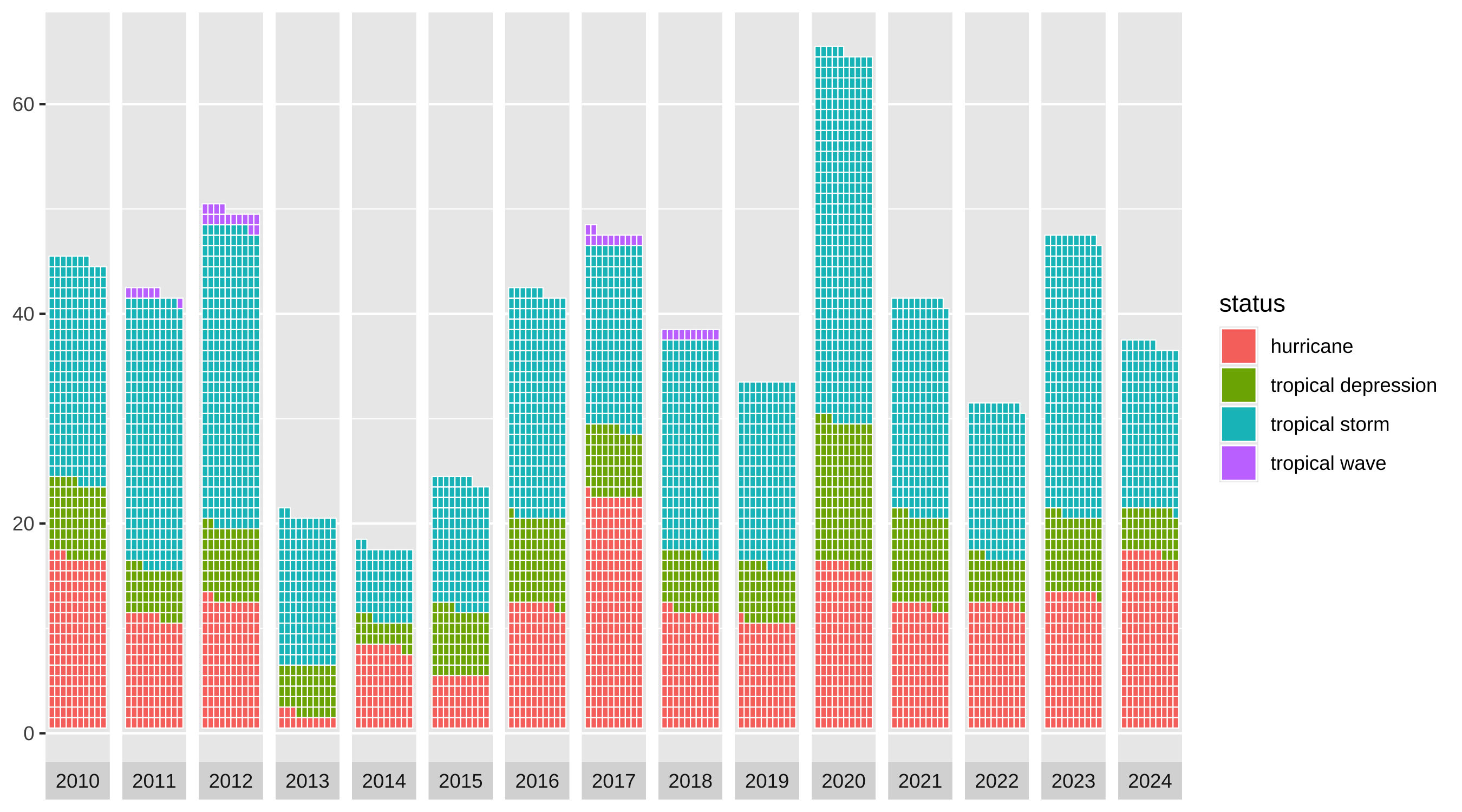
w3 <- w2 +
  facet_wrap(~year, nrow = 1, strip.position = "bottom") +
  scale_x_discrete()
w3

4. Square squares

coord_equal() keeps the tiles from stretching, and the y-axis labels are multiplied by ten so the axis counts storms rather than rows of squares.

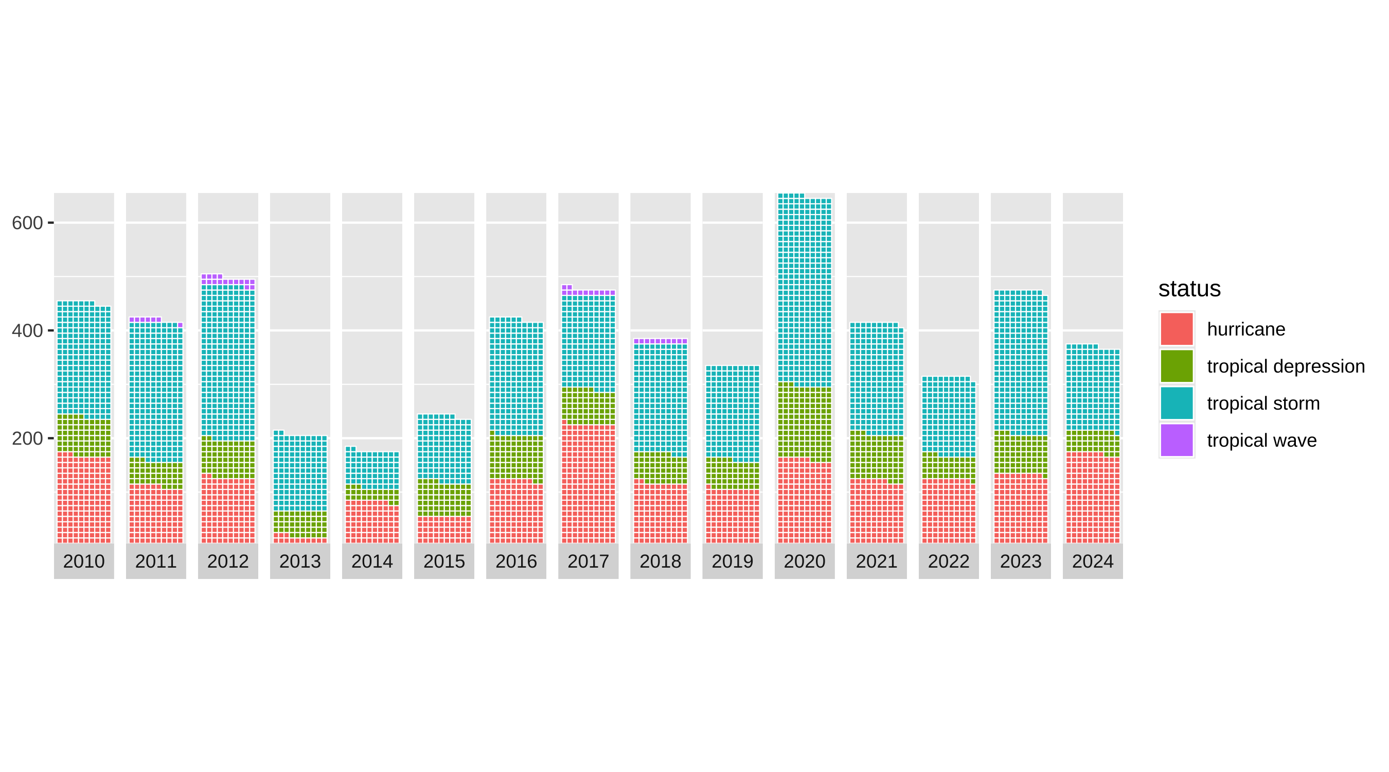
w4 <- w3 +
  scale_y_continuous(labels = function(x) x * 10, expand = c(0, 0)) +
  coord_equal()
w4

5. Colour

The four storm categories are coloured with the Hiroshige palette from MetBrewer.

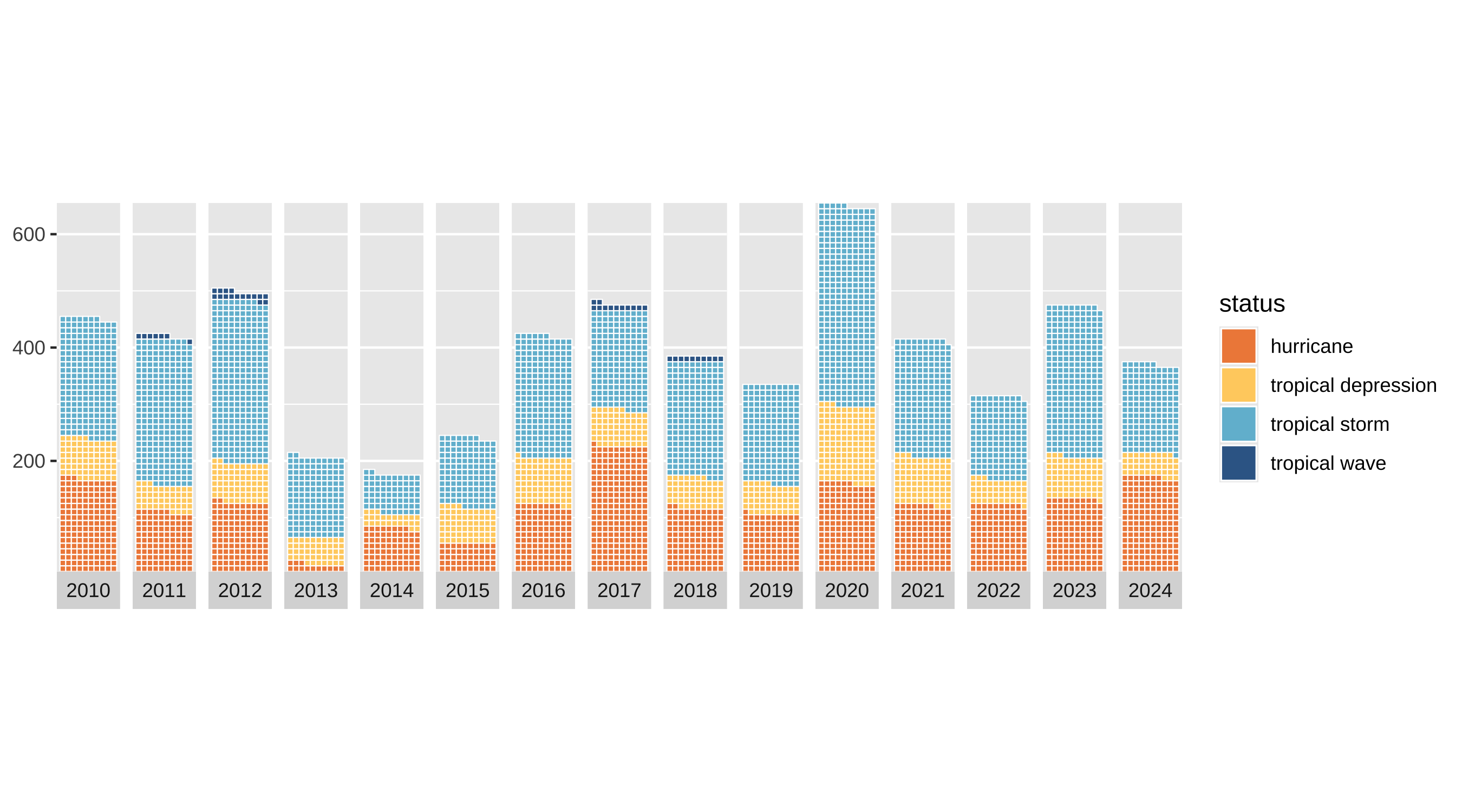
w5 <- w4 +
  MetBrewer::scale_fill_met_d("Hiroshige", direction = 1)
w5

6. Text

The title states the finding outright rather than describing the chart, with the definition of a tropical storm carried in the subtitle.

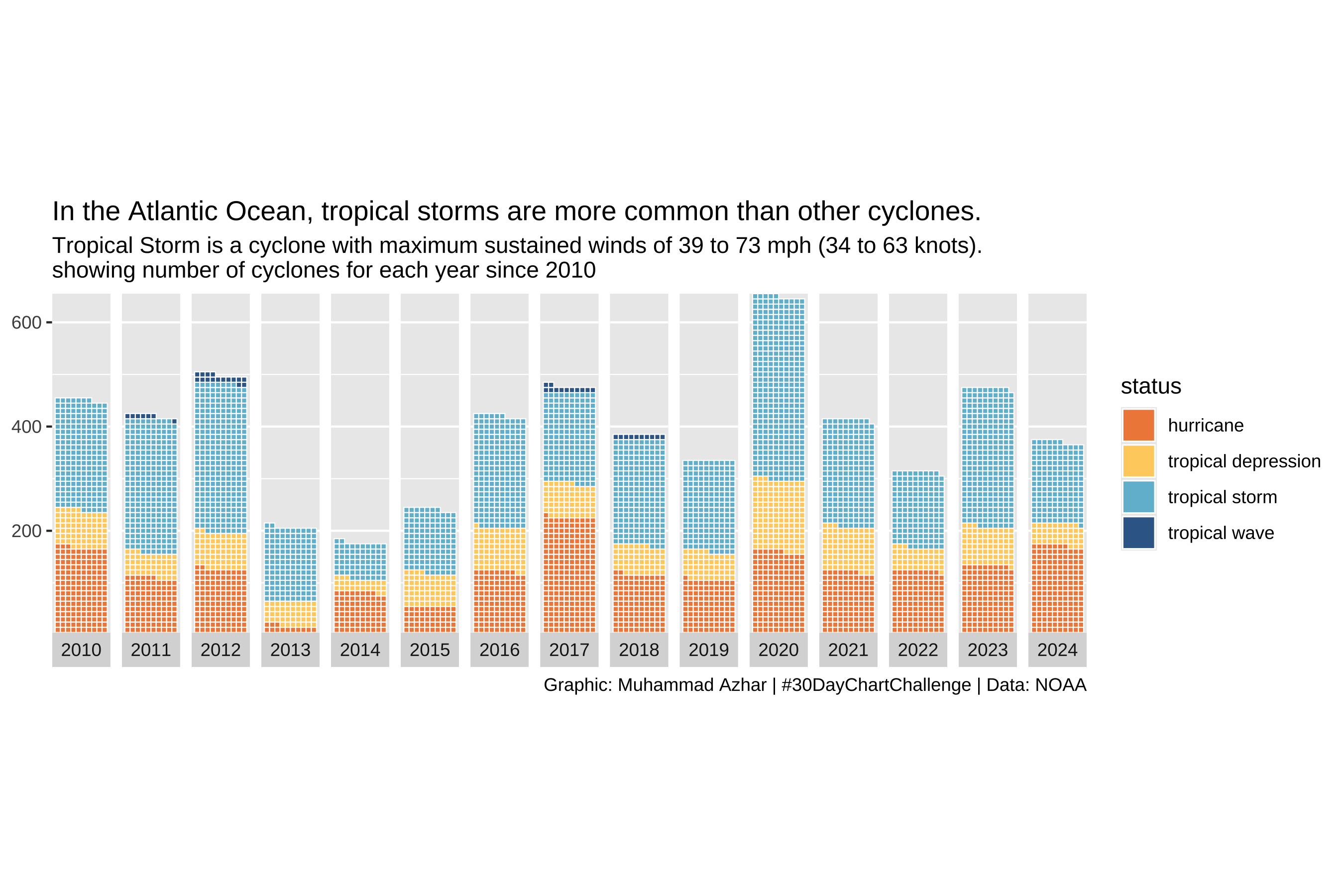
w6 <- w5 +
  labs(title = title_text,
       subtitle = subtitle_text,
       caption = caption_text)
w6

7. Theme

The last step does the most visible work: Outfit and Cabin from Google Fonts, no axis titles, the legend moved to the top with squarish keys, and a white background with generous margins.

w6 +
  theme_minimal() +
  theme(
    axis.title = element_blank(),
    axis.text.x = element_text(family = body_font, size = 12),
    axis.text.y = element_text(family = body_font, size = 12),
    legend.position = "top",
    legend.title = element_blank(),
    legend.spacing = unit(0.5, 'cm'),
    legend.key.height = unit(0.5, 'cm'),
    legend.key.width = unit(0.7, 'cm'),
    legend.text = element_text(family = body_font, size = 13, face = 'plain', color = "grey10"),
    plot.title.position = "plot",
    plot.title = element_textbox(margin = margin(20, 0, 10, 0), size = 30,
                                 family = title_font, face = "bold", width = unit(55, "lines")),
    plot.subtitle = element_text(margin = margin(10, 0, 20, 0), size = 16,
                                 family = body_font, color = "grey15"),
    plot.caption = element_text(family = body_font, face = "plain", size = 14,
                                color = "grey40", hjust = .5, margin = margin(20, 0, 0, 0)),
    plot.background = element_rect(color = "white", fill = "white"),
    plot.margin = margin(20, 40, 20, 40)
  )