Subway table (gt)

NoteCredit

This is a rebuild of a table originally created by Karina Bartolomé: The grammar of tables · source code. All credit for the original design goes to the author.

It uses the real Buenos Aires subway geography (station coordinates and the city’s barrios polygons) with placeholder passenger numbers, and brings back the per-line inline graphics from the original: a polar clock plot of hourly use, a map with station points sized by passenger share, a stacked time-of-day bar, and a daily evolution line.

A summary of subway use in Buenos Aires
Real geography, placeholder passenger data (styled after 'The grammar of tables')
Line	Route	Most used station	Use per hour	Number of passengers		Morning||Afternoon||Night	Passengers per day
			Passengers per hour	Total
A	Plaza de Mayo - San Pedrito	Carabobo		7.68M	−9.5%
B	Alem - J. M. de Rosas	Florida		10.40M	15.9%
C	Retiro - Constitución	Retiro		2.88M	−11.5%
D	Catedral - Congreso de Tucumán	Bulnes		5.68M	0.4%
E	Bolívar - Plaza de los Virreyes	Correo Central		6.03M	−5.2%
H	Facultad de Derecho - Hospitales	Venezuela		4.59M	−9.0%
Placeholder rebuild of a table by Karina Bartolomé. Geography: Open Data Portal, Autonomous City of Buenos Aires; passenger figures are simulated.

library(gt)
library(gtExtras)
library(dplyr)
library(tidyr)
library(purrr)
library(ggplot2)
library(sf)

here <- function(...) file.path("data", ...)

# Buenos Aires subway lines and their official colors
line_colors <- c(
  A = "#18cccc", B = "#eb0909", C = "#233aa8",
  D = "#02db2e", E = "#c618cc", H = "#ffdd00"
)

# --- Real geography -------------------------------------------------------
map_caba <- st_read(here("barrios.geojson"), quiet = TRUE)

stations <- readr::read_csv(here("stations.csv"), show_col_types = FALSE) |>
  rename(line = linea, station = estacion) |>
  filter(line %in% names(line_colors))

set.seed(42)

# --- Placeholder passenger data -------------------------------------------
# Per-station total passengers for the month
stations <- stations |>
  mutate(pax_station = round(runif(n(), 5e4, 6e5)))

# Hourly distribution per line (a plausible double-peaked commuter shape)
base_hour <- dnorm(0:23, 8, 2) + 0.8 * dnorm(0:23, 18, 2.5) + 0.05
hourly <- map_dfr(names(line_colors), function(ln) {
  w <- base_hour * runif(24, 0.7, 1.3)
  tibble(line = ln, hour = 0:23, pax_total = round(w / sum(w) * 4e6))
})

# Daily evolution per line across the month
daily <- map_dfr(names(line_colors), function(ln) {
  d <- seq(as.Date("2021-11-01"), as.Date("2021-11-30"), by = "day")
  wk <- ifelse(format(d, "%u") %in% c("6", "7"), 0.45, 1)
  tibble(line = ln, date = d,
         pax_total = round(wk * runif(length(d), 8e4, 1.3e5)))
})

# Circular mean hour, weighted by passengers (replaces the {circular} pkg)
mean_hours <- hourly |>
  group_by(line) |>
  summarise(
    mean_hour = {
      ang <- hour / 24 * 2 * pi
      m <- atan2(sum(pax_total * sin(ang)), sum(pax_total * cos(ang)))
      (m / (2 * pi) * 24) %% 24
    },
    .groups = "drop"
  )

# --- Plot builders (ported from the original R code) ----------------------
fig_clock_plot <- function(.line) {
  mean_hour <- mean_hours$mean_hour[mean_hours$line == .line]
  temp <- hourly |>
    filter(line == .line) |>
    mutate(color_hour = hour == round(mean_hour))
  ggplot(temp, aes(hour, pax_total)) +
    geom_col(color = "white", fill = "lightgrey") +
    coord_polar(start = 0) +
    geom_vline(xintercept = mean_hour, color = line_colors[[.line]], linewidth = 2) +
    geom_label(
      aes(y = max(pax_total) + quantile(pax_total, 0.3),
          color = color_hour, label = hour),
      size = 6, label.size = NA, show.legend = FALSE
    ) +
    scale_color_manual(values = c("black", line_colors[[.line]])) +
    scale_x_continuous("", limits = c(0, 24), breaks = 0:24) +
    scale_y_continuous(labels = scales::unit_format(unit = "K", scale = 1e-3)) +
    labs(y = NULL) +
    theme_minimal() +
    theme(text = element_text(size = 22, color = "grey"),
          axis.text.x = element_blank(), panel.grid = element_blank())
}

fig_map <- function(.line) {
  temp <- stations |>
    filter(line == .line) |>
    mutate(pax_percent = pax_station / sum(pax_station))
  ggplot() +
    geom_sf(data = map_caba, color = "black", fill = "white", linewidth = 0.1) +
    geom_point(
      data = temp, aes(long, lat, size = pax_percent),
      alpha = 0.7, fill = line_colors[[.line]], color = "black", shape = 21
    ) +
    scale_size_continuous(range = c(1, 9), guide = "none") +
    theme_void()
}

fig_evol <- function(.line) {
  ggplot(filter(daily, line == .line), aes(date, pax_total)) +
    geom_line(color = "grey", linewidth = 2.5) +
    geom_line(color = line_colors[[.line]], linewidth = 1.5) +
    scale_y_continuous(labels = scales::unit_format(unit = "K", scale = 1e-3)) +
    labs(x = NULL, y = NULL) +
    theme_minimal() +
    theme(text = element_text(size = 22),
          panel.grid = element_blank(), axis.text.x = element_blank())
}

# --- One row per line -----------------------------------------------------
tbl_data <- stations |>
  group_by(line) |>
  summarise(
    most_used_station = station[which.max(pax_station)],
    pax_total = sum(pax_station),
    .groups = "drop"
  ) |>
  mutate(
    variation = runif(n(), -0.12, 0.18),
    route = c(
      "Plaza de Mayo - San Pedrito", "Alem - J. M. de Rosas",
      "Retiro - Constitución", "Catedral - Congreso de Tucumán",
      "Bolívar - Plaza de los Virreyes", "Facultad de Derecho - Hospitales"
    ),
    # placeholder text columns; ggplots are injected via text_transform below
    clock_plot = "", passengers_per_day = "", map = ""
  ) |>
  rowwise() |>
  mutate(passengers_type = list(as.numeric(round(prop.table(runif(3)) * 100)))) |>
  ungroup() |>
  select(line, route, most_used_station, clock_plot, pax_total, variation,
         passengers_type, passengers_per_day, map)

# ggplot objects held separately, in table row order
clock_plots <- map(tbl_data$line, fig_clock_plot)
evol_plots   <- map(tbl_data$line, fig_evol)
map_plots    <- map(tbl_data$line, fig_map)
tbl_data |>
  gt() |>
  tab_header(
    title = md("**A summary of subway use in Buenos Aires**"),
    subtitle = "Real geography, placeholder passenger data (styled after 'The grammar of tables')"
  ) |>
  opt_align_table_header("left") |>
  tab_spanner(label = "Use per hour", columns = clock_plot) |>
  tab_spanner(label = "Number of passengers", columns = c(pax_total, variation)) |>
  cols_align("center", columns = c(pax_total, variation, most_used_station)) |>
  cols_width(
    line ~ px(50), route ~ px(150), most_used_station ~ px(110),
    clock_plot ~ px(150), pax_total ~ px(80), variation ~ px(80),
    passengers_type ~ px(120), passengers_per_day ~ px(150), map ~ px(120)
  ) |>
  # color each line label
  {\(x) Reduce(function(tbl, ln) {
    tab_style(tbl, cell_text(color = line_colors[[ln]], weight = "bold"),
              cells_body(columns = line, rows = line == ln))
  }, names(line_colors), x)}() |>
  tab_style(cell_fill(color = "#f0f0f0"), cells_body(columns = route)) |>
  fmt_number(pax_total, suffixing = TRUE) |>
  fmt_percent(variation, decimals = 1) |>
  text_transform(
    locations = cells_body(columns = clock_plot),
    fn = function(x) map(clock_plots, ggplot_image, height = px(120), aspect_ratio = 1)
  ) |>
  text_transform(
    locations = cells_body(columns = passengers_per_day),
    fn = function(x) map(evol_plots, ggplot_image, height = px(90), aspect_ratio = 2)
  ) |>
  text_transform(
    locations = cells_body(columns = map),
    fn = function(x) map(map_plots, ggplot_image, height = px(120), aspect_ratio = 0.9)
  ) |>
  gt_plt_bar_stack(
    column = passengers_type, position = "fill",
    labels = c("Morning", "Afternoon", "Night"),
    palette = c("grey", "#A3B1C9", "#4C699E"),
    fmt_fn = scales::label_percent(scale = 1), width = 60
  ) |>
  cols_label(
    line = "Line", route = "Route", most_used_station = "Most used station",
    clock_plot = md("Passengers per hour"), pax_total = md("Total"),
    variation = md("% Variation"), passengers_per_day = md("Passengers per day"),
    map = md("% Passengers per station")
  ) |>
  tab_source_note(md(paste0(
    "Placeholder rebuild of a table by Karina Bartolomé. Geography: Open Data ",
    "Portal, Autonomous City of Buenos Aires; passenger figures are simulated."
  ))) |>
  tab_options(
    data_row.padding = px(2),
    table.border.top.style = "hidden",
    table.border.bottom.style = "hidden"
  )

How it is built, step by step

Each tab adds one piece of the recipe on top of the previous one, so you can see what every part of the finished table contributes. The code for each step is shown below its output.

1. One row per line

Everything starts from a six-row summary, one row per subway line. The clock_plot, passengers_per_day and map columns are deliberately empty strings: they are placeholders whose contents get swapped for images later.

# A tibble: 6 × 5
  line  route                            most_used_station pax_total variation
  <chr> <chr>                            <chr>                 <dbl>     <dbl>
1 A     Plaza de Mayo - San Pedrito      Carabobo            7675481  -0.0948 
2 B     Alem - J. M. de Rosas            Florida            10398294   0.159  
3 C     Retiro - Constitución            Retiro              2880562  -0.115  
4 D     Catedral - Congreso de Tucumán   Bulnes              5679157   0.00423
5 E     Bolívar - Plaza de los Virreyes  Correo Central      6027375  -0.0519 
6 H     Facultad de Derecho - Hospitales Venezuela           4585029  -0.0901 

tbl_data |>
  select(line, route, most_used_station, pax_total, variation)

2. The inline plots

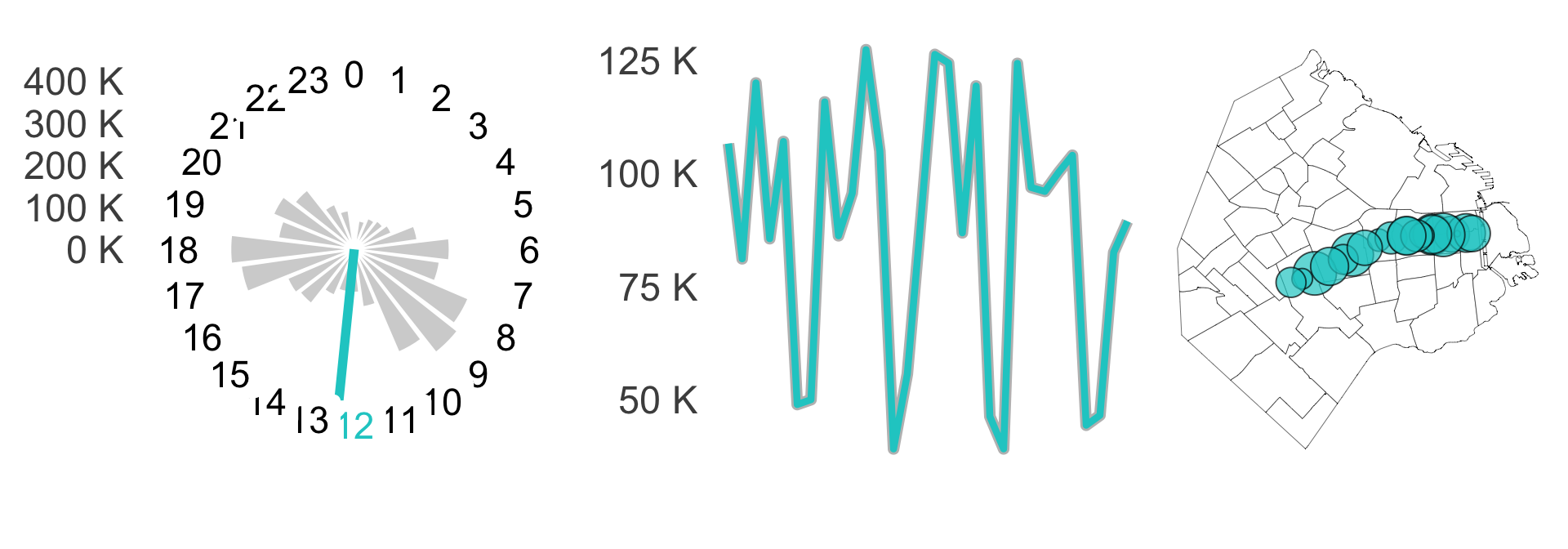
Each graphic is an ordinary standalone ggplot, built by a function that takes a line name. They are stripped down hard (no axis text, no legend) because they will be rendered a few dozen pixels tall. Here are all three for line A.

library(patchwork)
fig_clock_plot("A") + fig_evol("A") + fig_map("A")

3. A bare gt table

gt() on its own already gives a competent table. Everything from here is narrowing what the reader has to work to see.

line	route	most_used_station	clock_plot	pax_total	variation	passengers_per_day	map
A	Plaza de Mayo - San Pedrito	Carabobo		7675481	-0.09483455
B	Alem - J. M. de Rosas	Florida		10398294	0.15904011
C	Retiro - Constitución	Retiro		2880562	-0.11506554
D	Catedral - Congreso de Tucumán	Bulnes		5679157	0.00422772
E	Bolívar - Plaza de los Virreyes	Correo Central		6027375	-0.05190717
H	Facultad de Derecho - Hospitales	Venezuela		4585029	-0.09010782

t3 <- tbl_data |>
  select(-passengers_type) |>
  gt()
t3

4. Structure

A left-aligned title, spanners that group related columns under one heading, and explicit column widths. Fixing the widths matters here because the image columns have no natural size of their own.

A summary of subway use in Buenos Aires
Real geography, placeholder passenger data (styled after 'The grammar of tables')
line	route	most_used_station	Use per hour	Number of passengers		passengers_type	passengers_per_day	map
			clock_plot	pax_total	variation
A	Plaza de Mayo - San Pedrito	Carabobo		7675481	-0.09483455	24, 32, 45
B	Alem - J. M. de Rosas	Florida		10398294	0.15904011	24, 56, 20
C	Retiro - Constitución	Retiro		2880562	-0.11506554	33, 10, 57
D	Catedral - Congreso de Tucumán	Bulnes		5679157	0.00422772	57, 5, 37
E	Bolívar - Plaza de los Virreyes	Correo Central		6027375	-0.05190717	23, 40, 38
H	Facultad de Derecho - Hospitales	Venezuela		4585029	-0.09010782	42, 32, 26

t4 <- tbl_data |>
  gt() |>
  tab_header(
    title = md("**A summary of subway use in Buenos Aires**"),
    subtitle = "Real geography, placeholder passenger data (styled after 'The grammar of tables')"
  ) |>
  opt_align_table_header("left") |>
  tab_spanner(label = "Use per hour", columns = clock_plot) |>
  tab_spanner(label = "Number of passengers", columns = c(pax_total, variation)) |>
  cols_align("center", columns = c(pax_total, variation, most_used_station)) |>
  cols_width(
    line ~ px(50), route ~ px(150), most_used_station ~ px(110),
    clock_plot ~ px(150), pax_total ~ px(80), variation ~ px(80),
    passengers_type ~ px(120), passengers_per_day ~ px(150), map ~ px(120)
  )
t4

5. Colour and number formatting

Each line label is painted in that line’s official colour by folding tab_style() over the six lines, the route column gets a light fill to set it apart from the numbers, and the totals and variations are formatted as suffixed numbers and percentages.

A summary of subway use in Buenos Aires
Real geography, placeholder passenger data (styled after 'The grammar of tables')
line	route	most_used_station	Use per hour	Number of passengers		passengers_type	passengers_per_day	map
			clock_plot	pax_total	variation
A	Plaza de Mayo - San Pedrito	Carabobo		7.68M	−9.5%	24, 32, 45
B	Alem - J. M. de Rosas	Florida		10.40M	15.9%	24, 56, 20
C	Retiro - Constitución	Retiro		2.88M	−11.5%	33, 10, 57
D	Catedral - Congreso de Tucumán	Bulnes		5.68M	0.4%	57, 5, 37
E	Bolívar - Plaza de los Virreyes	Correo Central		6.03M	−5.2%	23, 40, 38
H	Facultad de Derecho - Hospitales	Venezuela		4.59M	−9.0%	42, 32, 26

t5 <- t4 |>
  {\(x) Reduce(function(tbl, ln) {
    tab_style(tbl, cell_text(color = line_colors[[ln]], weight = "bold"),
              cells_body(columns = line, rows = line == ln))
  }, names(line_colors), x)}() |>
  tab_style(cell_fill(color = "#f0f0f0"), cells_body(columns = route)) |>
  fmt_number(pax_total, suffixing = TRUE) |>
  fmt_percent(variation, decimals = 1)
t5

6. Injecting the plots

text_transform() replaces the contents of each placeholder column with images rendered from the ggplot lists via gt::ggplot_image(). The lists are in table row order, which is the only thing keeping plots matched to their line.

A summary of subway use in Buenos Aires
Real geography, placeholder passenger data (styled after 'The grammar of tables')
line	route	most_used_station	Use per hour	Number of passengers		passengers_type	passengers_per_day	map
			clock_plot	pax_total	variation
A	Plaza de Mayo - San Pedrito	Carabobo		7.68M	−9.5%	24, 32, 45
B	Alem - J. M. de Rosas	Florida		10.40M	15.9%	24, 56, 20
C	Retiro - Constitución	Retiro		2.88M	−11.5%	33, 10, 57
D	Catedral - Congreso de Tucumán	Bulnes		5.68M	0.4%	57, 5, 37
E	Bolívar - Plaza de los Virreyes	Correo Central		6.03M	−5.2%	23, 40, 38
H	Facultad de Derecho - Hospitales	Venezuela		4.59M	−9.0%	42, 32, 26

t6 <- t5 |>
  text_transform(
    locations = cells_body(columns = clock_plot),
    fn = function(x) map(clock_plots, ggplot_image, height = px(120), aspect_ratio = 1)
  ) |>
  text_transform(
    locations = cells_body(columns = passengers_per_day),
    fn = function(x) map(evol_plots, ggplot_image, height = px(90), aspect_ratio = 2)
  ) |>
  text_transform(
    locations = cells_body(columns = map),
    fn = function(x) map(map_plots, ggplot_image, height = px(120), aspect_ratio = 0.9)
  )
t6

7. Stacked bars

gtExtras::gt_plt_bar_stack() turns the list column of three numbers per row into a labelled, filled bar, so the morning/afternoon/night split needs no separate legend.

A summary of subway use in Buenos Aires
Real geography, placeholder passenger data (styled after 'The grammar of tables')
line	route	most_used_station	Use per hour	Number of passengers		Morning||Afternoon||Night	passengers_per_day	map
			clock_plot	pax_total	variation
A	Plaza de Mayo - San Pedrito	Carabobo		7.68M	−9.5%
B	Alem - J. M. de Rosas	Florida		10.40M	15.9%
C	Retiro - Constitución	Retiro		2.88M	−11.5%
D	Catedral - Congreso de Tucumán	Bulnes		5.68M	0.4%
E	Bolívar - Plaza de los Virreyes	Correo Central		6.03M	−5.2%
H	Facultad de Derecho - Hospitales	Venezuela		4.59M	−9.0%

t7 <- t6 |>
  gt_plt_bar_stack(
    column = passengers_type, position = "fill",
    labels = c("Morning", "Afternoon", "Night"),
    palette = c("grey", "#A3B1C9", "#4C699E"),
    fmt_fn = scales::label_percent(scale = 1), width = 60
  )
t7

8. Labels and finishing

Readable column labels, the source note that flags the passenger figures as simulated, tight row padding, and hidden outer borders.

A summary of subway use in Buenos Aires
Real geography, placeholder passenger data (styled after 'The grammar of tables')
Line	Route	Most used station	Use per hour	Number of passengers		Morning||Afternoon||Night	Passengers per day
			Passengers per hour	Total
A	Plaza de Mayo - San Pedrito	Carabobo		7.68M	−9.5%
B	Alem - J. M. de Rosas	Florida		10.40M	15.9%
C	Retiro - Constitución	Retiro		2.88M	−11.5%
D	Catedral - Congreso de Tucumán	Bulnes		5.68M	0.4%
E	Bolívar - Plaza de los Virreyes	Correo Central		6.03M	−5.2%
H	Facultad de Derecho - Hospitales	Venezuela		4.59M	−9.0%
Placeholder rebuild of a table by Karina Bartolomé. Geography: Open Data Portal, Autonomous City of Buenos Aires; passenger figures are simulated.

t7 |>
  cols_label(
    line = "Line", route = "Route", most_used_station = "Most used station",
    clock_plot = md("Passengers per hour"), pax_total = md("Total"),
    variation = md("% Variation"), passengers_per_day = md("Passengers per day"),
    map = md("% Passengers per station")
  ) |>
  tab_source_note(md(paste0(
    "Placeholder rebuild of a table by Karina Bartolomé. Geography: Open Data ",
    "Portal, Autonomous City of Buenos Aires; passenger figures are simulated."
  ))) |>
  tab_options(
    data_row.padding = px(2),
    table.border.top.style = "hidden",
    table.border.bottom.style = "hidden"
  )