Brussels health-precarity map

NoteCredit

This recreates the building-level map from Bruxelles malade, a data-journalism investigation by the Belgian cooperative magazine Médor. The original is a scroll-driven D3/Mapbox map; here it is rebuilt in R from the same underlying data (the article’s own building-footprint and per-sector data files). All credit for the reporting and design goes to Médor.

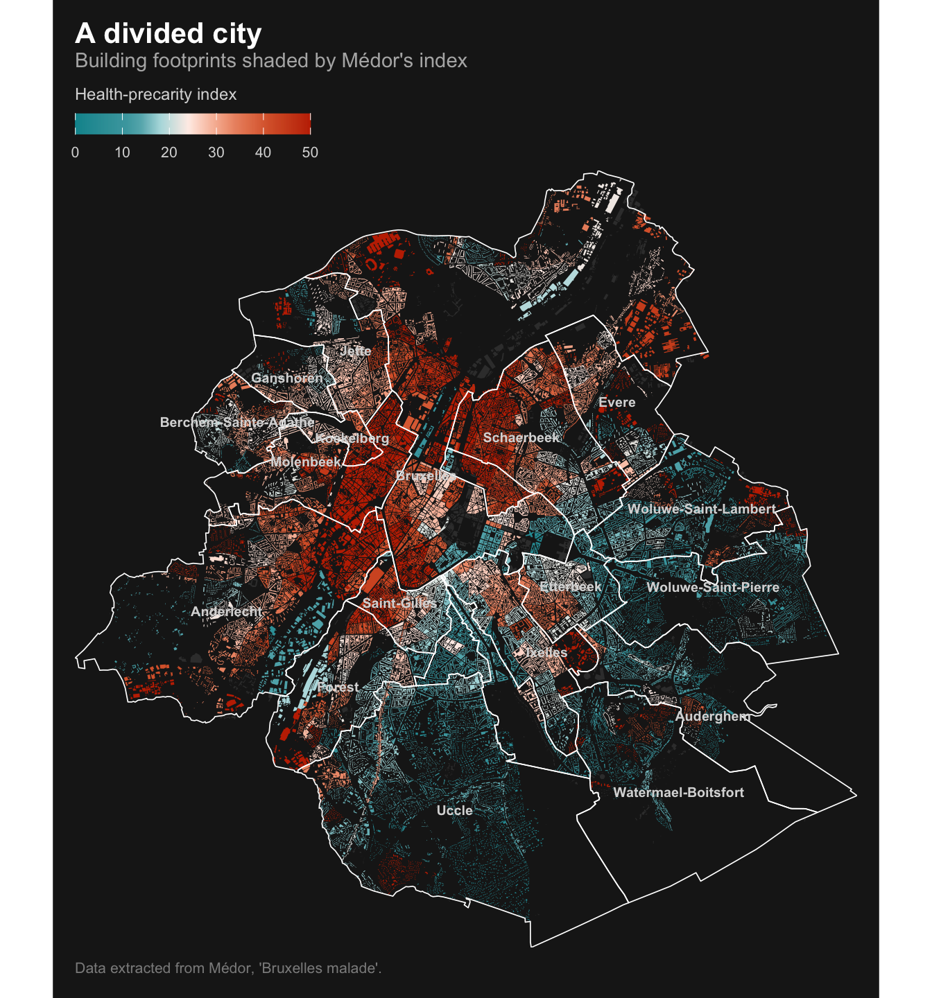
The original shades Brussels’ building footprints by a health-precarity index (dim) on a dark basemap. Since the piece is not written in R, I extracted its merged-buildings geometry (721 dissolved footprints, one per statistical sector, each carrying its dim value) and rebuilt the map with sf and ggplot2, reusing Médor’s exact color ramp. Higher values (red) mean more precarious; lower values (teal) mean better off. Hover over a district to highlight it and see its area-weighted average index (rendered interactively with ggiraph).

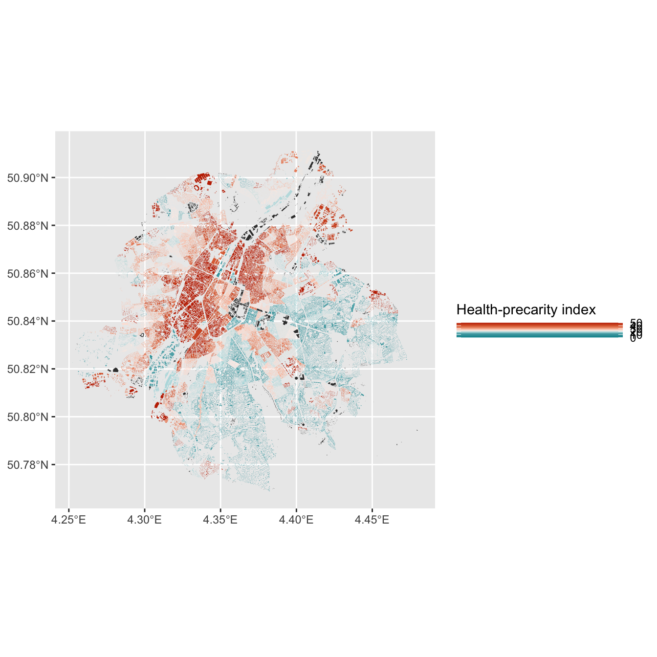
The pattern is the article’s central finding: a “poor croissant” of high-index (red) neighbourhoods curls through the inner-city and industrial west (Molenbeek, Anderlecht, Saint-Josse), while the wealthier south-east (Uccle, Woluwe) sits at the teal end. The extracted per-sector data also carries the other indicators used in the piece (air pollution no2/pm25, green coverage, noise, diabetes rates, cancer-screening uptake), so the same footprints can be recolored by any of them.

library(sf)
library(dplyr)
library(ggplot2)
library(scales)
library(ggiraph)
crs_local <- 3812 # Belgian Lambert 2008

# Building footprints, each carrying the precarity index `dim`
buildings <- read_sf(file.path("choropleth-data", "bxlBuildings.topo.json")) |>
  st_set_crs(4326) |>
  st_transform(crs_local) |>
  # the sector code's first 5 digits are the commune (NIS) code
  mutate(commune_code = substr(sector, 1, 5),
         area = as.numeric(st_area(geometry)))

# Commune outlines + labels, dissolved from the statistical sectors
sectors <- read_sf(file.path("choropleth-data", "brusselsSectors.json")) |>
  st_set_crs(4326) |>
  st_transform(crs_local) |>
  st_make_valid() |>
  mutate(commune_code = substr(cd_sector, 1, 5))

communes <- sectors |>
  group_by(commune_code, commune = tx_munty_descr_fr) |>
  summarise(.groups = "drop")

# Area-weighted average index per district (commune)
district_dim <- buildings |>
  st_drop_geometry() |>
  filter(!is.na(dim)) |>
  group_by(commune_code) |>
  summarise(dim_district = weighted.mean(dim, area), .groups = "drop")

communes <- communes |>
  left_join(district_dim, by = "commune_code") |>
  mutate(tooltip = sprintf("%s\nPrecarity index: %.1f", commune, dim_district),
         label_pt = st_point_on_surface(geometry))

# Médor's diverging ramp with the article's exact break points (dim 0 -> 50)
stops <- c(0, 11, 14, 18, 24, 29, 34, 41, 50)
cols  <- c("#00939C", "#49A6AE", "#65B3BA", "#B2DCDF", "#FEEEE8",
           "#F8C0AA", "#EC9370", "#DA6436", "#C22E00")

bg <- "#1b1b1b"

p <- ggplot() +
  geom_sf(data = buildings, aes(fill = dim), color = NA) +
  # interactive district layer: transparent until hovered
  geom_sf_interactive(
    data = communes,
    aes(tooltip = tooltip, data_id = commune_code),
    fill = "transparent", color = "white", linewidth = 0.3
  ) +
  geom_sf_text(data = communes, aes(label = commune, geometry = label_pt),
               color = "grey85", size = 2.6, fontface = "bold", check_overlap = TRUE) +
  scale_fill_gradientn(
    colours = cols,
    values = rescale(stops, from = c(0, 50)),
    limits = c(0, 50), oob = squish,
    na.value = "#3a3a3a",
    name = "Health-precarity index",
    guide = guide_colourbar(barwidth = unit(45, "mm"), barheight = unit(4, "mm"),
                            title.position = "top", ticks = FALSE)
  ) +
  labs(
    title = "A divided city",
    subtitle = "Building footprints shaded by Médor's index — hover a district for its average",
    caption = "Data extracted from Médor, 'Bruxelles malade'."
  ) +
  coord_sf(expand = FALSE) +
  theme_void(base_size = 13) +
  theme(
    plot.background = element_rect(fill = bg, color = NA),
    panel.background = element_rect(fill = bg, color = NA),
    legend.position = "top",
    legend.justification = "left",
    legend.title = element_text(color = "grey85", size = 9),
    legend.text = element_text(color = "grey85", size = 8),
    plot.title = element_text(face = "bold", color = "white", margin = margin(b = 2)),
    plot.subtitle = element_text(color = "grey70", size = 11, margin = margin(b = 8)),
    plot.caption = element_text(color = "grey55", size = 8, hjust = 0, margin = margin(t = 8)),
    plot.margin = margin(12, 12, 12, 12)
  )

girafe(
  ggobj = p,
  width_svg = 8.5, height_svg = 9,
  options = list(
    opts_hover(css = "fill:#ffffff55;stroke:white;stroke-width:1.5px;"),
    opts_tooltip(css = "background:#1b1b1b;color:white;padding:6px 10px;border-radius:4px;font-family:sans-serif;font-size:12px;white-space:pre;"),
    opts_toolbar(saveaspng = FALSE),
    opts_sizing(rescale = TRUE)
  )
)

How it is built, step by step

Each tab adds one layer of the recipe on top of the previous one, so you can see what every piece of the final map contributes. The code for each step is shown below its plot.

1. The geometry

The extracted footprints are one dissolved polygon per statistical sector, each carrying its precarity index. Reprojecting to Belgian Lambert 2008 (EPSG:3812) is what lets areas be measured in metres for the weighted averages later.

Simple feature collection with 5 features and 4 fields
Geometry type: MULTIPOLYGON
Dimension:     XY
Bounding box:  xmin: 649160.6 ymin: 662037.4 xmax: 653864.1 ymax: 676549.2
Projected CRS: ETRS89 / Belgian Lambert 2008
# A tibble: 5 × 5
  sector    commune_code   dim    area                                  geometry
  <chr>     <chr>        <dbl>   <dbl>                        <MULTIPOLYGON [m]>
1 21016A214 21016         16.6  13468. (((650239.5 665856.3, 650264.4 665862.1,…
2 21005A322 21005         81.4   1600. (((651418.2 668120.7, 651456 668075.6, 6…
3 21015A33- 21015         36.3  42855. (((650841.3 671842.5, 650818.3 671832.1,…
4 21016A342 21016          4.1 207838. (((650972.6 662044.7, 650958.4 662037.4,…
5 21004G30- 21004         25.3  83727. (((653228.5 675861.2, 653216 675867.3, 6…

buildings |>
  select(sector, commune_code, dim, area) |>
  head(5)

2. Footprints

A single geom_sf() with no outline colour. At this zoom the footprints read as texture rather than individual buildings, which is the effect the original is after.

m2 <- ggplot() +
  geom_sf(data = buildings, aes(fill = dim), color = NA)
m2

3. Médor’s colour ramp

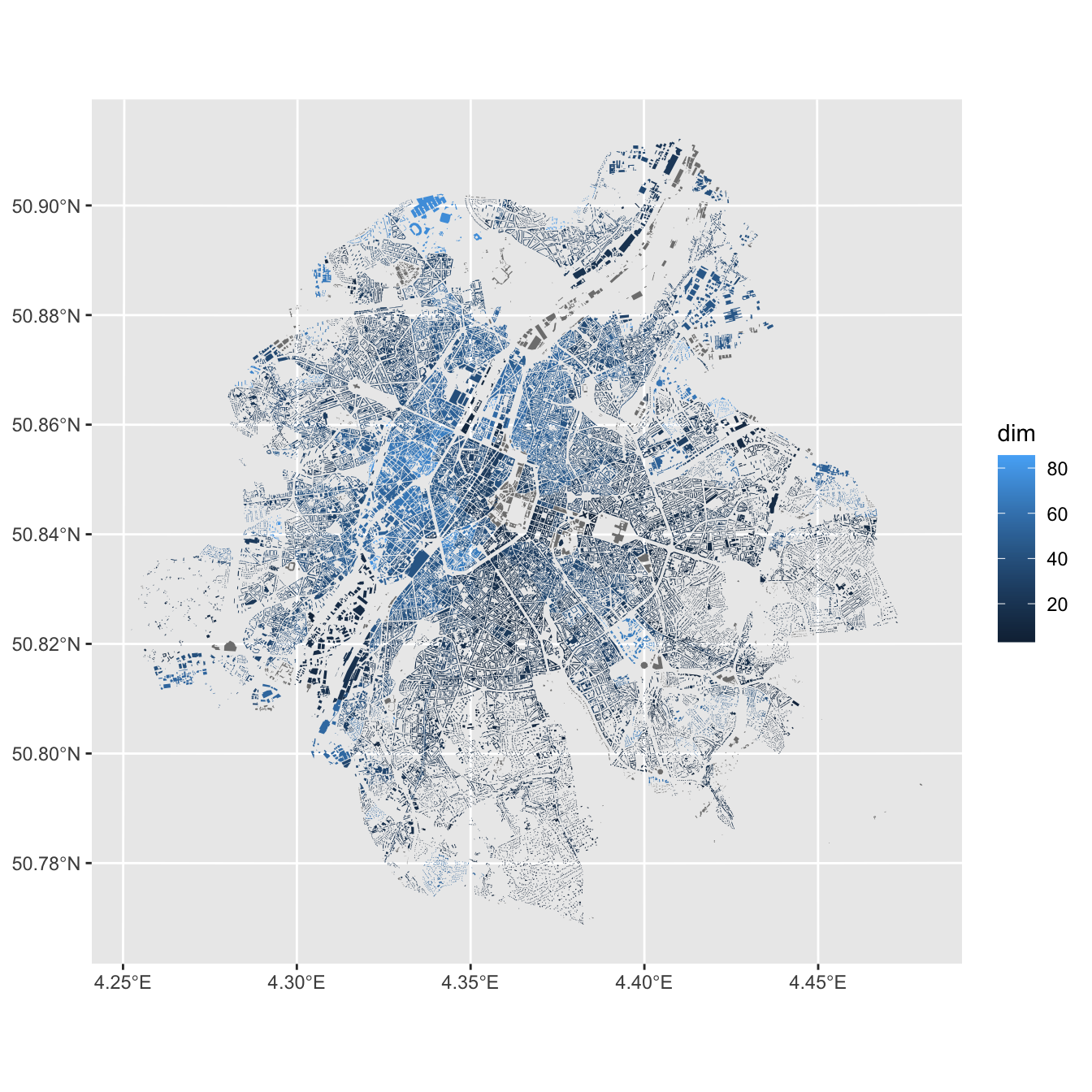
The default blue gradient hides the story. scale_fill_gradientn() with the article’s nine stops and colours puts the neutral cream tone at the middle of the index, so teal and red read as “better off” and “more precarious”.

m3 <- m2 +
  scale_fill_gradientn(
    colours = cols,
    values = rescale(stops, from = c(0, 50)),
    limits = c(0, 50), oob = squish,
    na.value = "#3a3a3a",
    name = "Health-precarity index",
    guide = guide_colourbar(barwidth = unit(45, "mm"), barheight = unit(4, "mm"),
                            title.position = "top", ticks = FALSE)
  )
m3

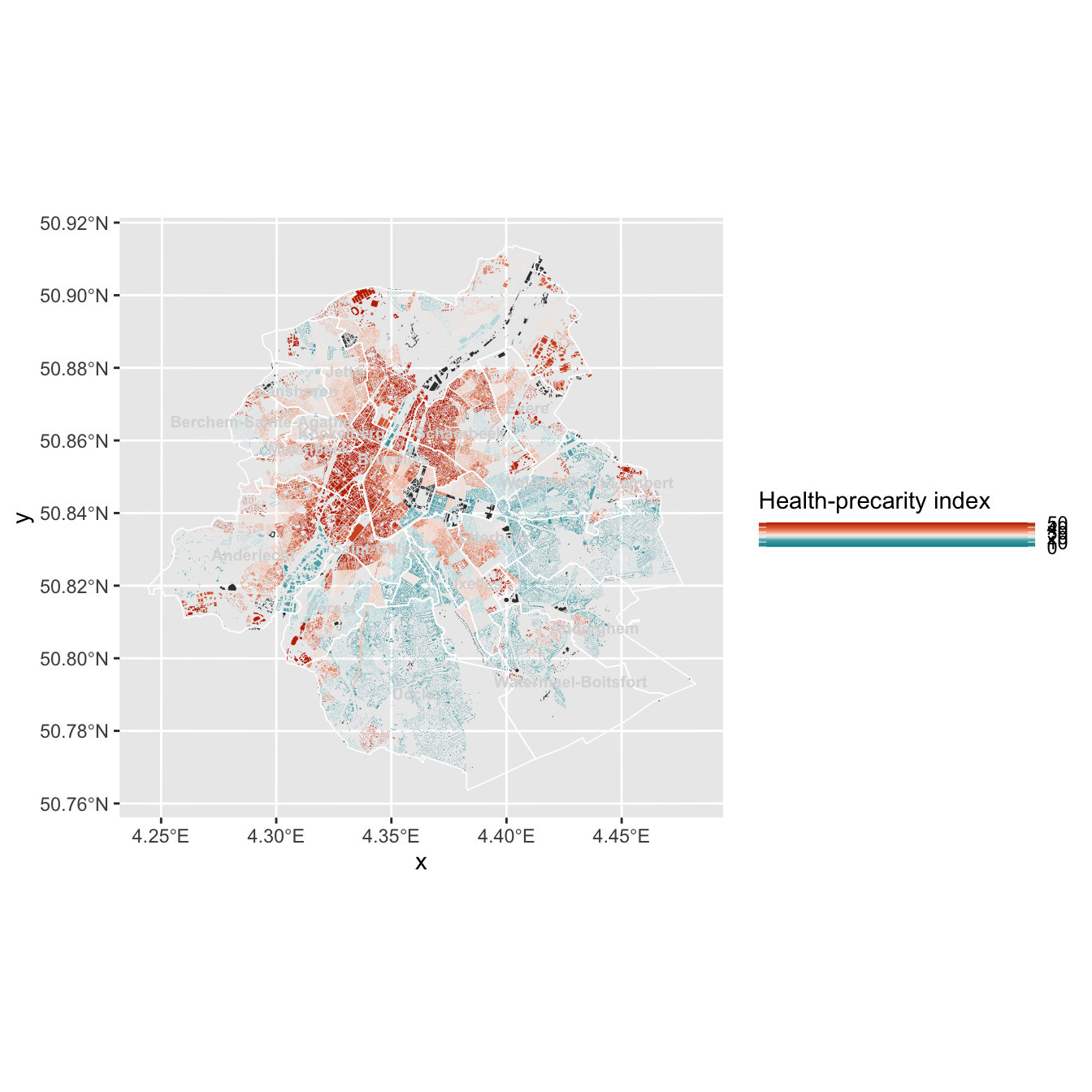
4. District outlines

The commune boundaries and their names give the reader somewhere to stand. The outline layer is geom_sf_interactive() with a transparent fill: it is invisible until hovered, when it becomes the highlight and tooltip target.

m4 <- m3 +
  geom_sf_interactive(
    data = communes,
    aes(tooltip = tooltip, data_id = commune_code),
    fill = "transparent", color = "white", linewidth = 0.3
  ) +
  geom_sf_text(data = communes, aes(label = commune, geometry = label_pt),
               color = "grey85", size = 2.6, fontface = "bold", check_overlap = TRUE)
m4

5. Dark theme

theme_void() strips the axes and graticule, and the near-black background is what makes the ramp glow the way the original does. The legend sits top-left, above the map.

m5 <- m4 +
  labs(
    title = "A divided city",
    subtitle = "Building footprints shaded by Médor's index",
    caption = "Data extracted from Médor, 'Bruxelles malade'."
  ) +
  coord_sf(expand = FALSE) +
  theme_void(base_size = 13) +
  theme(
    plot.background = element_rect(fill = bg, color = NA),
    panel.background = element_rect(fill = bg, color = NA),
    legend.position = "top",
    legend.justification = "left",
    legend.title = element_text(color = "grey85", size = 9),
    legend.text = element_text(color = "grey85", size = 8),
    plot.title = element_text(face = "bold", color = "white", margin = margin(b = 2)),
    plot.subtitle = element_text(color = "grey70", size = 11, margin = margin(b = 8)),
    plot.caption = element_text(color = "grey55", size = 8, hjust = 0, margin = margin(t = 8)),
    plot.margin = margin(12, 12, 12, 12)
  )
m5

6. Interactivity

Nothing above is interactive yet: it is a static ggplot with interactive aesthetics recorded on the district layer. ggiraph::girafe() renders it to SVG and wires those up, with the hover CSS supplying the white wash.

girafe(
  ggobj = m5,
  width_svg = 8.5, height_svg = 9,
  options = list(
    opts_hover(css = "fill:#ffffff55;stroke:white;stroke-width:1.5px;"),
    opts_tooltip(css = "background:#1b1b1b;color:white;padding:6px 10px;border-radius:4px;font-family:sans-serif;font-size:12px;white-space:pre;"),
    opts_toolbar(saveaspng = FALSE),
    opts_sizing(rescale = TRUE)
  )
)