AWS, CSV Input, SageMaker Endpoint

csv

vetiver

Amazon SageMaker

AWS

Using vetiver to version a model on Amazon SageMaker as an endpoint, and predict from it

Note

This page was last generated on 2024-02-29. If you find the code out of date please file an issue.

Changes from standard

All changes from the standard pipeline are highlighted with a cranberry line to the right.

Loading packages

We are using the tidymodels package to do the modeling, embed for target encoding, pins for versioning, vetiver for version and deployment, and smdocker for deploying to SageMaker.

# install.packages("pak")
# pak::pak("tidymodels", "embed", "vetiver", "pins", "smdocker")
library(tidymodels)
library(embed)
library(vetiver)
library(pins)
library(smdocker)

Loading Data

We are using the smaller laxflights2022 data set described on the data preparation page.

flights <- readr::read_csv(here::here("data/laxflights2022_lite.csv"))

glimpse(flights)

Rows: 3,757
Columns: 8
$ arr_delay <dbl> 4, -15, -12, 38, -9, -17, 5, 12, -40, 6, -7, 28, 25, -9, 180…
$ dep_delay <dbl> 9, -8, 0, -7, 3, 6, 29, -1, 2, 7, 6, 13, 34, -2, 191, 52, 9,…
$ carrier   <chr> "UA", "OO", "AA", "UA", "OO", "OO", "UA", "AA", "DL", "DL", …
$ tailnum   <chr> "N37502", "N198SY", "N410AN", "N77261", "N402SY", "N509SY", …
$ origin    <chr> "LAX", "LAX", "LAX", "LAX", "LAX", "LAX", "LAX", "LAX", "LAX…
$ dest      <chr> "KOA", "EUG", "HNL", "DEN", "FAT", "SFO", "MCO", "MIA", "OGG…
$ distance  <dbl> 2504, 748, 2556, 862, 209, 337, 2218, 2342, 2486, 862, 156, …
$ time      <dttm> 2022-01-01 13:15:00, 2022-01-01 14:00:00, 2022-01-01 14:45:…

Modeling

As a reminder, the modeling task we are trying to accomplish is the following:

Given all the information we have, from the moment the plane leaves for departure. Can we predict the arrival delay arr_delay?

Our outcome is arr_delay and the remaining variables are predictors. We will be fitting an xgboost model as a regression model.

Splitting Data

Since the data set is already in chronological order, we can create a time split of the data using initial_time_split(), this will put the first 75% of the data into the training data set, and the remaining 25% into the testing data set.

set.seed(1234)

flights_split <- initial_time_split(flights, prop = 3/4)
flights_training <- training(flights_split)

Since we are doing hyperparameter tuning, we will also be creating a cross-validation split

flights_folds <- vfold_cv(flights_training)

Feature Engineering

We need to do a couple of things to make this data set work for our model. The datetime variable time needs to be transformed, as does the categorical variables carrier, tailnum, origin and dest.

From the time variable, the month and day of the week are extracted as categorical variables, then the day of year and time of day are extracted as numerics. The origin and dest variables will be turned into dummy variables, and carrier, tailnum, time_month, and time_dow will be converted to numerics with likelihood encoding.

flights_rec <- recipe(arr_delay ~ ., data = flights_training) %>%
  step_novel(all_nominal_predictors()) %>%
  step_other(origin, dest, threshold = 0.025) %>%
  step_dummy(origin, dest) %>%
  step_date(time, 
            features = c("month", "dow", "doy"), 
            label = TRUE, 
            keep_original_cols = TRUE) %>%
  step_time(time, features = "decimal_day", keep_original_cols = FALSE) %>%
  step_lencode_mixed(all_nominal_predictors(), outcome = vars(arr_delay)) %>%
  step_zv(all_predictors())

Specifying Models

We will be fitting a boosted tree model in the form of a xgboost model.

xgb_spec <-
  boost_tree(
    trees = tune(),
    min_n = tune(),
    mtry = tune(),
    learn_rate = 0.01
  ) %>%
  set_engine("xgboost") %>%
  set_mode("regression")

xgb_wf <- workflow(flights_rec, xgb_spec)

Hyperparameter Tuning

doParallel::registerDoParallel()

xgb_rs <- tune_grid(
  xgb_wf,
  resamples = flights_folds,
  grid = 10
)

i Creating pre-processing data to finalize unknown parameter: mtry

We can visualize the performance of the different hyperparameter selections

autoplot(xgb_rs)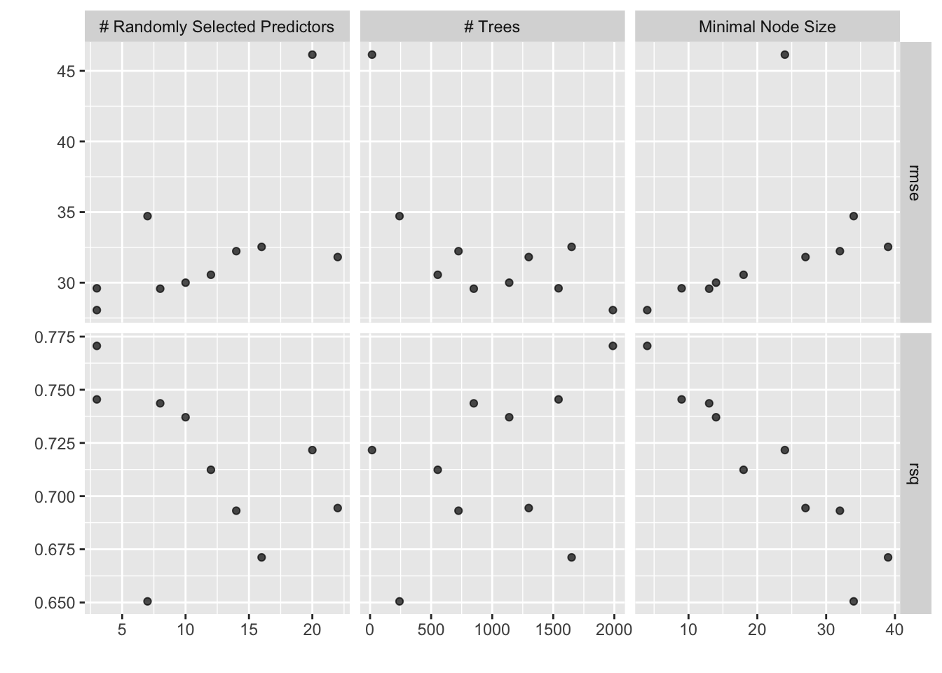

and look at the top result

show_best(xgb_rs, metric = "rmse")

# A tibble: 5 × 9
   mtry trees min_n .metric .estimator  mean     n std_err .config              
  <int> <int> <int> <chr>   <chr>      <dbl> <int>   <dbl> <chr>                
1     3  1988     4 rmse    standard    28.1    10    5.88 Preprocessor1_Model01
2     8   849    13 rmse    standard    29.6    10    6.44 Preprocessor1_Model04
3     3  1543     9 rmse    standard    29.6    10    6.11 Preprocessor1_Model02
4    10  1139    14 rmse    standard    30.0    10    6.44 Preprocessor1_Model05
5    12   554    18 rmse    standard    30.6    10    6.77 Preprocessor1_Model06

Fitting Final Model

Once we are satisfied with the modeling that has been done, we can fit our final model. We use finalize_workflow() to use the best hyperparameters, and last_fit() to fit the model to the training data set and evaluate it on the testing data set.

xgb_last <- xgb_wf %>%
  finalize_workflow(select_best(xgb_rs, metric = "rmse")) %>%
  last_fit(flights_split)

Creating vetiver model

v <- xgb_last %>%
  extract_workflow() %>%
  vetiver_model("flights_xgb")
v


── flights_xgb ─ <bundled_workflow> model for deployment 
A xgboost regression modeling workflow using 7 features

Version model with pins on Amazon SageMaker

We will version this model on Amazon S3 using the pins package.

For the smoothest experience, we recommend that you authenticate using environment variables. The two variables you will need are AWS_ACCESS_KEY_ID and AWS_SECRET_ACCESS_KEY.

Warning

Depending on your S3 setup, you will need to use additional variables to connect. Please see https://github.com/paws-r/paws/blob/main/docs/credentials.md and this pins issue for help if the following paragraphs doesn’t work for you.

Tip

The function usethis::edit_r_environ() can be very handy to open .Renviron file to specify your environment variables.

You can find both of these keys in the same location.

Open the AWS Console
Click on your username near the top right and select Security Credentials
Click on Users in the sidebar
Click on your username
Click on the Security Credentials tab
Click Create Access Key
Click Show User Security Credentials

Once you have those two, you can add them to your .Renviron file in the following format:

AWS_SECRET_ACCESS_KEY=xxxxxxxxxxxxxxxxxxxxxxxxxxxx
AWS_ACCESS_KEY_ID=xxxxxxxxxxxxxxxxxxxxxxxxxxxx

Note that you don’t want to put quotes around the values.

Once that is all done, we can create a board that connects to Amazon S3, and write our vetiver model to the board. Now that you have set up the environment variables, we can create a pins board. When using S3 you need to specify a bucket and its region. This cannot be done with Pins and has to be done beforehand.

board <- board_s3(
  "tidymodels-pipeline-example",
  region = "us-west-1"
)
vetiver_pin_write(board, v)

Since we are using vetiver_deploy_sagemaker() which uses the {smdocker} package, we need to make sure that we have the right authetication and settings.

If you are working locally, you will likely need to explicitly set up your execution role to work correctly. Check out Execution role requirements in the smdocker documentation, and especially note that the bucket containing your vetiver model needs to be added as a resource in your IAM role policy.

Once we are properly set up, we can use vetiver_deploy_sagemaker(), it takes a board, the name of endpoint and the instance_type Look at the Amazon SageMaker pricing to help you decide what you need. Depending on your model, it will take a little while to run as it installs what it needs.

new_endpoint <- vetiver_deploy_sagemaker(
  board = board,
  name = "flights_xgb",
  instance_type = "ml.t2.medium"
)

Make predictions from Connect endpoint

With the endpoint we can pass in some data set to predict with.

predict(
  new_endpoint,
  flights_training
)

# A tibble: 2,817 × 1
    .pred
    <dbl>
 1  -1.79
 2 -13.3 
 3 -17.3 
 4  -3.67
 5  82.8 
 6  52.2 
 7  10.7 
 8   8.04
 9  58.1 
10   5.39
# ℹ 2,807 more rows

:::