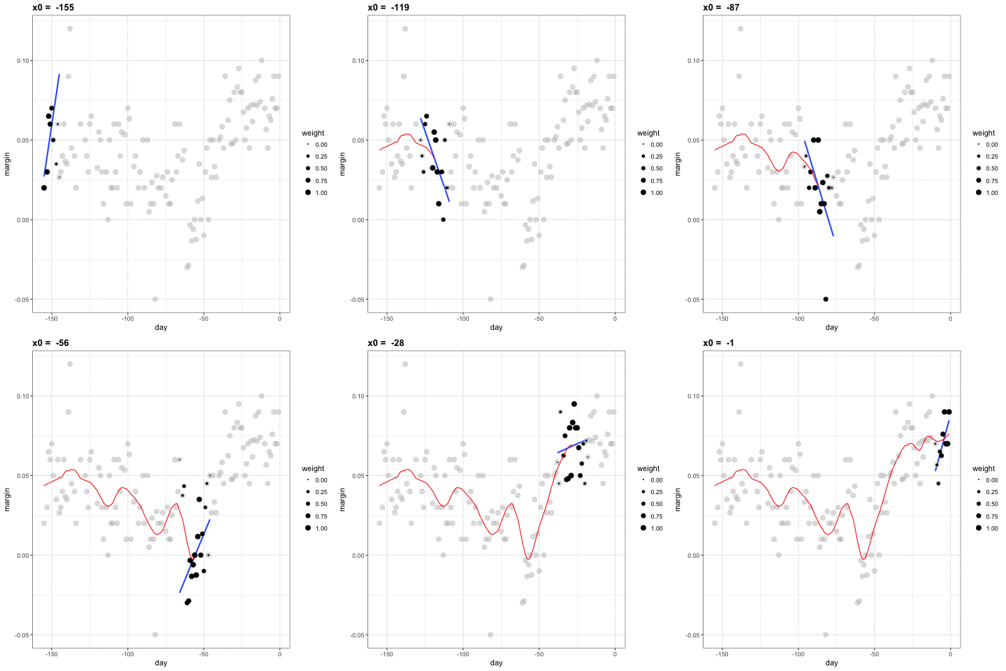
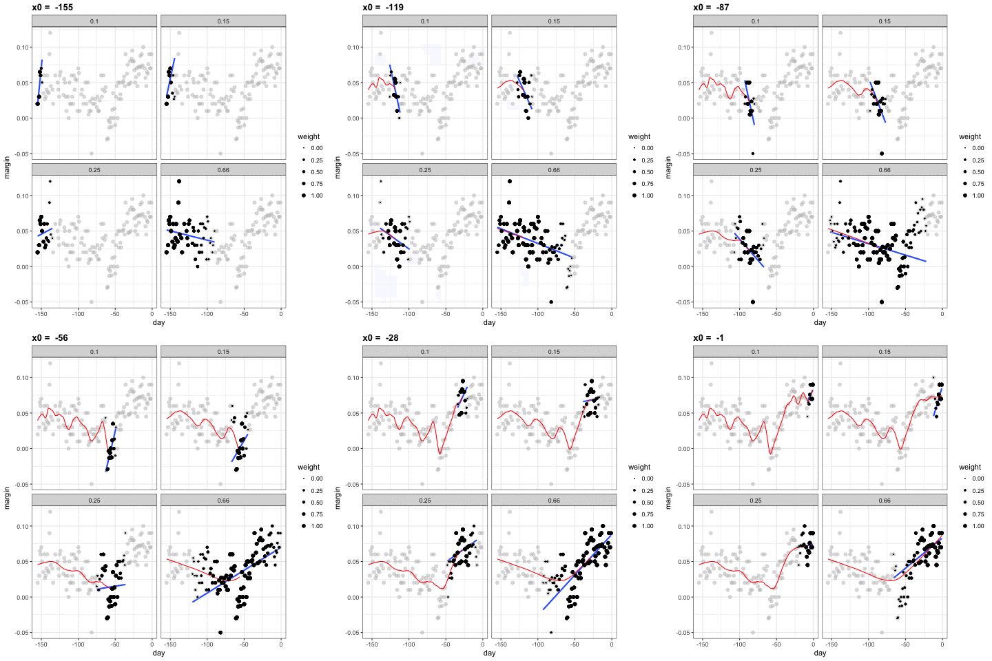
class: center, middle, title-slide # Moving Beyond Linearity ## AU STAT627 ### Emil Hvitfeldt ### 2022-03-28 --- <div style = "position:fixed; visibility: hidden"> `$$\require{color}\definecolor{orange}{rgb}{1, 0.603921568627451, 0.301960784313725}$$` `$$\require{color}\definecolor{blue}{rgb}{0.301960784313725, 0.580392156862745, 1}$$` `$$\require{color}\definecolor{pink}{rgb}{0.976470588235294, 0.301960784313725, 1}$$` </div> <script type="text/x-mathjax-config"> MathJax.Hub.Config({ TeX: { Macros: { orange: ["{\\color{orange}{#1}}", 1], blue: ["{\\color{blue}{#1}}", 1], pink: ["{\\color{pink}{#1}}", 1] }, loader: {load: ['[tex]/color']}, tex: {packages: {'[+]': ['color']}} } }); </script> <style> .orange {color: #FF9A4D;} .blue {color: #4D94FF;} .pink {color: #F94DFF;} </style> # Moving beyond Linearity We have so far worked (mostly) with linear models linear models are great because they are simple to describe, easy to work with in terms of interpretation and inference However, the linear assumption is often not satisfied This week we will see what happens once we slowly relax the linearity assumption --- # Moving beyond Linearity <img src="index_files/figure-html/unnamed-chunk-2-1.png" width="700px" style="display: block; margin: auto;" /> --- # Moving beyond Linearity <img src="index_files/figure-html/unnamed-chunk-3-1.png" width="700px" style="display: block; margin: auto;" /> --- # Moving beyond Linearity <img src="index_files/figure-html/unnamed-chunk-4-1.png" width="700px" style="display: block; margin: auto;" /> --- # Polynomial regression Simple linear regression `$$y_i = \beta_0 + \beta_1 x_i + \epsilon_i$$` 2nd-degree polynomial regression `$$y_i = \beta_0 + \beta_1 x_i + \beta_2 x_i^2 + \epsilon_i$$` --- # Polynomial regression Polynomial regression function with `\(d\)` degrees `$$y_i = \beta_0 + \beta_1 x_i + \beta_2 x_i^2 + \beta_3 x_i^3 + ... + \beta_d x_i^d + \epsilon_i$$` Notice how we can treat the polynomial regression as --- # Polynomial regression We are not limited to only use 1 variable when doing polynomial regression Instead of thinking of it as fitting a "polynomial regression" model Think of it as fitting a linear regression using polynomially expanded variables --- # Polynomial regression ### 2 degrees <img src="index_files/figure-html/unnamed-chunk-5-1.png" width="700px" style="display: block; margin: auto;" /> --- # Polynomial regression ### 3 degrees <img src="index_files/figure-html/unnamed-chunk-6-1.png" width="700px" style="display: block; margin: auto;" /> --- # Polynomial regression ### 4 degrees <img src="index_files/figure-html/unnamed-chunk-7-1.png" width="700px" style="display: block; margin: auto;" /> --- # Polynomial regression ### 10 degrees <img src="index_files/figure-html/unnamed-chunk-8-1.png" width="700px" style="display: block; margin: auto;" /> --- # Step Functions We can also try to turn continuous variables into categorical variables If we have data regarding the ages of people, then we can arrange the groups such as - under 21 - 21-34 - 35-49 - 50-65 - over 65 --- # Step Functions We divide a variable into multiple bins, constructing an ordered categorical variable --- # Step Functions <img src="index_files/figure-html/unnamed-chunk-9-1.png" width="700px" style="display: block; margin: auto;" /> --- # Step Functions <img src="index_files/figure-html/unnamed-chunk-10-1.png" width="700px" style="display: block; margin: auto;" /> --- # Step Functions <img src="index_files/figure-html/unnamed-chunk-11-1.png" width="700px" style="display: block; margin: auto;" /> --- # Step Functions <img src="index_files/figure-html/unnamed-chunk-12-1.png" width="700px" style="display: block; margin: auto;" /> --- # Step Functions Depending on the number of cuts, you might miss the action of the variable in question Be wary about using this method if you are going in blind, you end up creating a lot more columns of your data set, and your flexibility increase drastically --- # Basis Functions Both polynomial and piecewise-constant regression models are special cases of the **basis function** modeling approach The idea is to have a selection of functions `\(b_1(X), b_2(X), ..., b_K(X)\)` that we apply to our predictors `$$y_i = \beta_0 + \beta_1 b_1(x_i) + \beta_2 b_2(x_i) + \beta_3 b_3(x_i) + ... + \beta_K b_K(x_i) + \epsilon_i$$` Where `\(b_1(X), b_2(X), ..., b_K(X)\)` are fixed and known --- # Basis Functions The upside to this approach is that we can take advantage of the linear regression model for calculations along with all the inference tools and tests This does not mean that we are limited to using linear regression models when using basis functions --- # Regression Splines We can combine polynomial expansion and step functions to create **piecewise polynomials** Instead of fitting 1 polynomial over the whole range of the data, we can fit multiple polynomials in a piecewise manner --- # Regression Splines <img src="index_files/figure-html/unnamed-chunk-13-1.png" width="700px" style="display: block; margin: auto;" /> --- # Regression Splines <img src="index_files/figure-html/unnamed-chunk-14-1.png" width="700px" style="display: block; margin: auto;" /> --- # Regression Splines <img src="index_files/figure-html/unnamed-chunk-15-1.png" width="700px" style="display: block; margin: auto;" /> --- # Regression Splines <img src="index_files/figure-html/unnamed-chunk-16-1.png" width="700px" style="display: block; margin: auto;" /> --- # Local Regression **local regression** is a method where the modeling is happening locally namely, the fitted line only takes in information about nearby points --- # Local Regression .center[  ] --- # Local Regression .center[  ] --- # Generalized Additive Models Generalized Additive Models provide a general framework to extend the linear regression model by allowing non-linear functions of each predictor while maintaining additivity The standard multiple linear regression model `$$y_i = \beta_0 + \beta_1 x_{i1} + \beta_2 x_{i2} + ... + \beta_p x_{ip} + \epsilon_i$$` is extended by replacing each linear component `\(\beta_j x_{ij}\)` with a smooth linear function `\(f_j(x_{ij})\)` --- # Generalized Additive Models Given us `$$y_i = \beta_0 + f_1(x_{i1}) + f_2(x_{i2}) + f_3(x_{i3}) + ... + f_p(x_{ip}) + \epsilon_i$$` Since we are keeping the model additive we are left with a more interpretable model since we can look at the effect of each of the predictors on the response by keeping the other predictors constant --- # Pros and Cons Pro: GAMs allow us to fit a non-linear `\(f_j\)` to each `\(X_j\)`, so that we can automatically model non-linear relationships that standard linear regression will miss. This means that we do not need to manually try out many different transformations on each variable individually. --- # Pros and Cons Pro: The non-linear fits can potentially make more accurate predictions for the response `\(Y\)`. Pro: Because the model is additive, we can examine the effect of each `\(X_j\)` on `\(Y\)` individually while holding all of the other variables fixed. Pro: The smoothness of the function `\(f_j\)` for the variable `\(X_j\)` can be summarized via degrees of freedom. --- # Pros and Cons Con: The main limitation of GAMs is that the model is restricted to be additive. With many variables, important interactions can be missed. We can manually add interaction terms into the model by using appropriate pre-processing