Classification

Last we looked at regression tasks. In regression the response variable $Y$ is quantitative

In classification tasks, the response variable $Y$ is qualitative

This Difference will present some challenges we will cover this week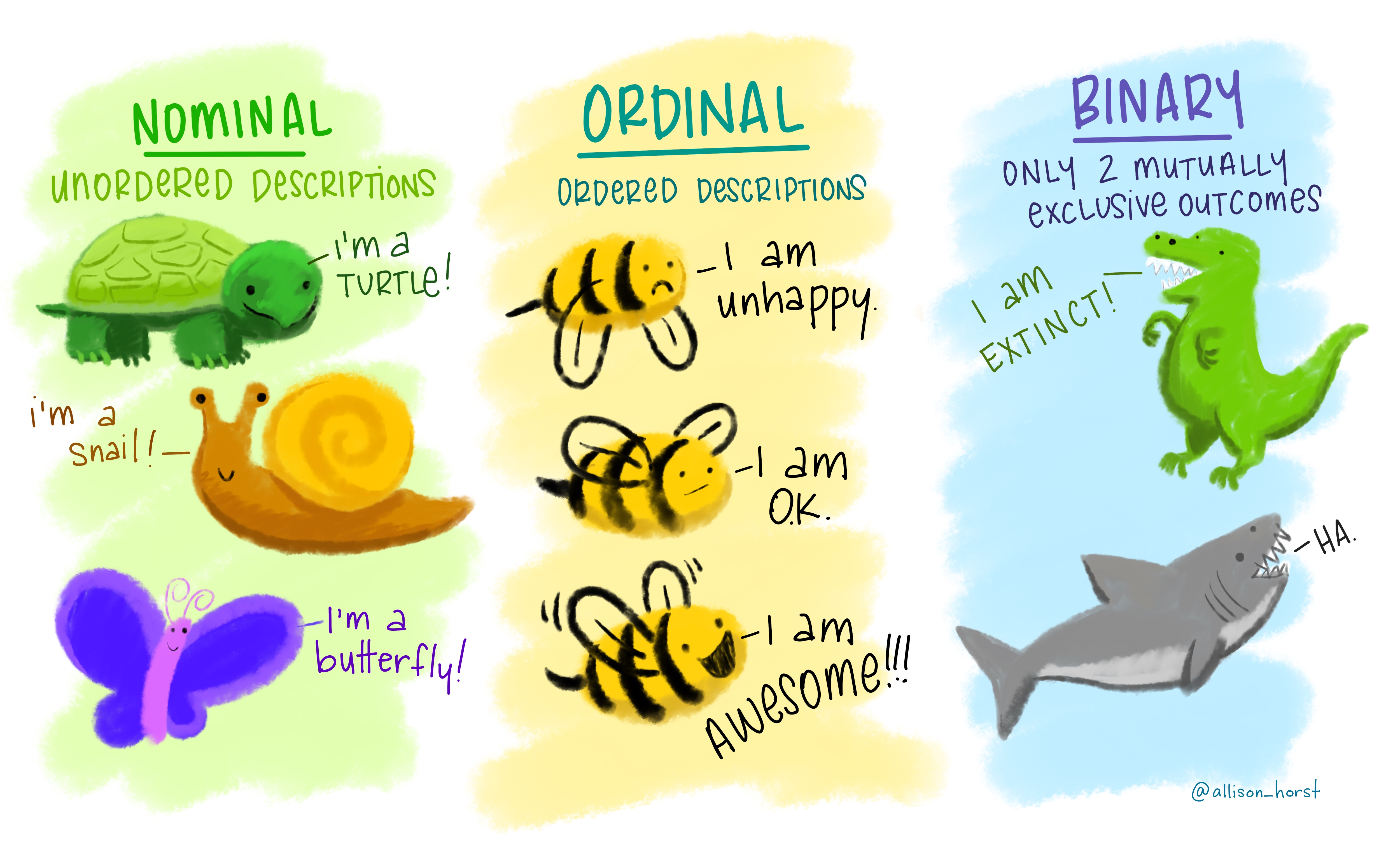

Examples of classification tasks

• Should we sent an email ad to this person?
• Are these symptoms indicative of cancer?
• Given an image, which fruit is depicted?

Two or more classes

There can be uncertainty

Can be more than one class at the same time

Classification visual

Classification visual - decision boundary

Classification visual

Classification visual - no hope

Nonlinear decision boundary

Logistic regression

conceptually creates a linear line separating 2 classes

Low flexibility, explainable method

(we will talk about LDA, QLA, and K-nearest neighbors on Wednesday)

Logistic regression

You might ask

• Why can't you use linear regression?

Response encoding

Propose we want to classify what kind of wine to market:

• red
• white

$Y$ has to be numeric for a linear model to work.

We could decode $red = 0, white = 1$.

but what would happen if we let $\hat{Y} >1$

Response encoding

What if we have more than 2 classes?

• red
• white
• rose
• dessert
• sparkling

We can't do $red = 1, white = 2, rose = 3, dessert = 4, sparking = 5$ because there isn't natural ordering and nothing to indicate that dessert wine is twice of white wine

Logistic regression

logistic (abstractly) models the probability that Y corresponds to a particular category

Now some mathematics!

The Logistic Model

We want to model the relationship between $p(X) = Pr(Y = 1|X)$ and $X$.

If we use a linear formulation

$$p(X) = \beta_0 + \beta_1X$$

then we will get negative probabilities which would be no good!

The Logistic Model

The Logistic Model

Using the logistic function gives us

$$p(X) = \dfrac{e^{\beta_0 + \beta_1X}}{1 + e^{\beta_0 + \beta_1X}}$$

Now no matter what the values of $X$, $\beta_0$ or $\beta_1$, $p(X)$ will always be contained between 0 and 1.

The Logistic Model

If we start with

$$p(X) = \dfrac{e^{\blue{\beta_0 + \beta_1X}}}{1 + e^{\blue{\beta_0 + \beta_1X}}}$$

and we see that this looks familiar, it is the linear combination we saw in linear regression we saw last week

Explain what the parameter estimates mean

odds

If we start with

$$p(X) = \dfrac{e^{\beta_0 + \beta_1X}}{1 + e^{\beta_0 + \beta_1X}}$$

after rearrangement gives

$$\dfrac{p(X)}{1 + p(X)} = e^{\beta_0 + \beta_1X}$$

odds

If we start with

$$p(X) = \dfrac{e^{\beta_0 + \beta_1X}}{1 + e^{\beta_0 + \beta_1X}}$$

after rearrangement gives

$$\orange{\dfrac{p(X)}{1 + p(X)}} = e^{\beta_0 + \beta_1X}$$

This is called the odds and can take any value between 0 and $\infty$.

log-odds

If we start with

$$p(X) = \dfrac{e^{\beta_0 + \beta_1X}}{1 + e^{\beta_0 + \beta_1X}}$$

after rearrangement gives

$$\dfrac{p(X)}{1 + p(X)} = e^{\beta_0 + \beta_1X}$$

taking the logarithm

$$\log\left(\dfrac{p(X)}{1 + p(X)}\right) = \beta_0 + \beta_1X$$

log-odds

$$\blue{\log\left(\dfrac{p(X)}{1 + p(X)}\right)} = \beta_0 + \beta_1X$$

The left-hand side is called the log-odds or logit.

How is this a classifier?

Logistic regression is not modeling classes

Logistic regression is modeling the probabilities that Y is equal on of the classes

Logistic regression turns into a classifier by picking a cutoff (usually 50%) and classifying according to this threshold.

Logistic regression decision boundary

Non-linear separator

Coefficients

Understanding:

Increasing $X$ by one unit changes the log odds by a factor of $e^{\beta_1}$

The amount of change in $p(X)$ depends on the current value of $X$

Making Predictions

Fitting the model gives us $\hat{\beta_0}$ and $\hat{\beta_1}$ which we can use to construct $\hat{p}(X)$

$$\hat{p}(X) = \dfrac{e^{\hat{\beta_0} + \hat{\beta_1}X}}{1 + e^{\hat{\beta_0} + \hat{\beta_1}X}}$$

Plugging in the values of $\hat{\beta_0}$, $\hat{\beta_1}$ and $X$ gives us a prediction

Example with penguins

library(palmerpenguins)
penguins2 <- penguins %>%
  mutate(species = factor(species == "Adelie", 
                          labels = c("Adelie", "Not Adelie")))
library(parsnip)
lr_spec <- logistic_reg() %>%
  set_engine("glm") %>%
  set_mode("classification")
lr_fit <- lr_spec %>%
  fit(species ~ bill_length_mm + bill_depth_mm + body_mass_g,
      data = penguins2)

Example with penguins

lr_fit

## parsnip model object
## 
## Fit time:  4ms 
## 
## Call:  stats::glm(formula = species ~ bill_length_mm + bill_depth_mm + 
##     body_mass_g, family = stats::binomial, data = data)
## 
## Coefficients:
##    (Intercept)  bill_length_mm   bill_depth_mm     body_mass_g  
##      32.965109       -4.903438        8.616116        0.006746  
## 
## Degrees of Freedom: 341 Total (i.e. Null);  338 Residual
##   (2 observations deleted due to missingness)
## Null Deviance:        469.4 
## Residual Deviance: 9.652     AIC: 17.65

Example with penguins

tidy(lr_fit)

## # A tibble: 4 x 5
##   term           estimate std.error statistic p.value
##   <chr>             <dbl>     <dbl>     <dbl>   <dbl>
## 1 (Intercept)    33.0      25.6          1.29  0.199 
## 2 bill_length_mm -4.90      2.65        -1.85  0.0647
## 3 bill_depth_mm   8.62      4.81         1.79  0.0733
## 4 body_mass_g     0.00675   0.00385      1.75  0.0800

Multi class classification

We have so far only talked about what happens with 2 classes

Logistic regression isn't able to work with multiple classes since it finds 1 best line to separate 2 classes

Logistic regression multiclass struggles

Logistic regression multiclass struggles

Evaluation

To evaluate a classifier we need to quantify how good and bad it is performing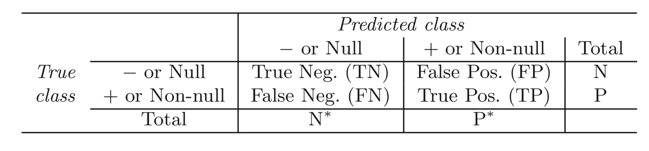

Different metrics will be different algebraic combinations of the above numbers

Evaluation metrics

Accuracy

$\dfrac{TN + TP}{TN + FN + FP + TP}$

Percentage of correct predictions

Drawback: If there are two classes A and B split 99% and 1%, you can get an accuracy of 99% by always predicting A

Evaluation metrics

Sensitivity

$\dfrac{TP}{FP + TP}$

Defined as the proportion of positive results out of the number of samples that were positive

Evaluation metrics

Specificity

$\dfrac{TP}{FP + TP}$

Measures the proportion of negatives that are correctly identified as negatives

ROC curve

Test-Train split

We have spent some time talking about fitting model and measuring performance

However, we need to be careful about how we go about that

performance metrics calculated on the data that was used to fit the data is likely to mislead

Test-Train split

In a prediction model, we are interested in the generalized performance. e.i. how well the model can perform on data it hasn't seen

Test-Train split

Test-Train split

We split the data into two groups (typically 75%/25%)

• training data set
• testing data set

We do the modeling on the training data set (it can be multiple models)

And then we use the testing data set ONCE to measure the performance

Why 75%/25%?

There are no real guidelines as to how you split the data

80/20 split is also used

It Will depend on data size

Why just once?

If you are working in a prediction setting, the testing data set represents fresh new data

If you modify your model you are essentially using information from the future to guide your modeling decisions

This is a kind of data-leakage and it will lead to overconfidence in the model and will come back to bite you once you start using the model

How will I be able to iterate?

We will talk more about how to efficiently use data in the next two weeks

How should we handle unbalanced classes?

How should we handle unbalanced classes?

How should we handle unbalanced classes?

stratified sampling

This stratification also works for regression tasks. The variable can be binned and samples to ensure equal distribution between training and testing data

There is very little downside to using stratified sampling.

More Data Leakage

Performing training-testing split in another place where data can leak

Any transformation done to the data should be done AFTER the split occurs as to not have had future information affect the modeling process

rsample

sample provides functionally to perform all different kinds of data splitting with a minimal footprint

rsample example

We bring back the penguins

penguins

## # A tibble: 344 x 8
##    species island    bill_length_mm bill_depth_mm flipper_length_mm body_mass_g
##    <fct>   <fct>              <dbl>         <dbl>             <int>       <int>
##  1 Adelie  Torgersen           39.1          18.7               181        3750
##  2 Adelie  Torgersen           39.5          17.4               186        3800
##  3 Adelie  Torgersen           40.3          18                 195        3250
##  4 Adelie  Torgersen           NA            NA                  NA          NA
##  5 Adelie  Torgersen           36.7          19.3               193        3450
##  6 Adelie  Torgersen           39.3          20.6               190        3650
##  7 Adelie  Torgersen           38.9          17.8               181        3625
##  8 Adelie  Torgersen           39.2          19.6               195        4675
##  9 Adelie  Torgersen           34.1          18.1               193        3475
## 10 Adelie  Torgersen           42            20.2               190        4250
## # … with 334 more rows, and 2 more variables: sex <fct>, year <int>

rsample example

Use initial_split() from rsample to generate a rsplit object

set.seed(1234) # remember the seed!
penguins_split <- initial_split(penguins)
penguins_split

## <Analysis/Assess/Total>
## <258/86/344>

This object store the information of what observations belong to each data set

rsample example

training() and testing() is used to extract the training data set and testing data set

set.seed(1234) # remember the seed!
penguins_split <- initial_split(penguins)
penquins_train <- training(penguins_split)
penquins_test <- testing(penguins_split)
dim(penquins_train)

## [1] 258   8

dim(penquins_test)

## [1] 86  8